Returns and Forecasting

Objective1: Find returns of NSE data>6months.having selected the 10th data as start and 95th data point as end.Also plot the assignment .

Solution:
Step 1: Read data  in the form of CSV file for the period 1/12/2011 to 5/02/2013
Command:
 z<-read.csv(file.choose(),header=T)

Step 2:Choose the Close column.
Command:
 close<-z$Close

Step 3:Vectorised the data i.e form a matrix of order 1X298 as 298 data points are available in close.
Command:
dim(close)<-c(1,298)

Step 4:Create time-series objects for close data from element (1,10 to1,95)
Command:
close.ts<-ts(close[1,10:95],deltat=1/252)
Step 5:Calculate difference between preceding and succeeding value
Command:
close.diff<-diff(close.ts)
Step 6: Calculate return :
Command:
return<-close.diff/lag(close.ts,k=-1)
final<-cbind(close.ts,close.diff,return)
Step 7: Plot
Command:
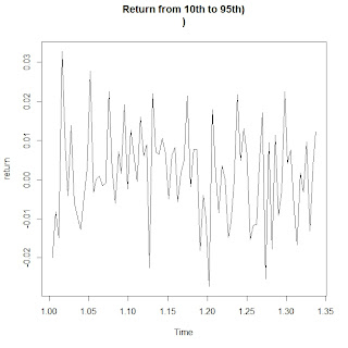
plot(return,main="Return from 10th to 95th")
plot(final,main="Data from 10th to 95, Difference, Return")

 Objective 2:1-700 data is available, Predict the data from 701-850, use the GLM estimation using LOGIT Analysis for the same

Step 1:Read data  in the form of CSV file

Command:
z<-read.csv(file.choose(),header=T)

Step 2:Check the dimension of z
Command
dim(z)


Step 3:Choose 1-700 data
Command

 new<-z[1:700,1:9]

Step 4:
Command
head(new)

Step 5:
Identify the factor and run the Logit regression
Command

 new$ed <- factor(new$ed)
 new.est<-glm(default ~ age + ed + employ + address + income, data=new, family ="binomial")
 summary(new.est)

Step 6
Prediction<-z[701:850,1:8]
 Prediction$ed<-factor(Prediction$ed)
 Prediction$prob<-predict(new.est, newdata =Prediction, type = "response")
 head(Prediction)